Genome Graphs
Metabolic networks have four columns. The first declares a unique name for the enzyme or enzymatic complex; the second declares a unique name for the reaction; the third column lists using comma unique names for substrates; and the last row list using comma unique names for products. To declare metabolites located at the periplasm or extracellular compartments, the user should employ the prefix “PER-” and “EX-”, respectively. Use spontaneous for non-enzymatic reactions.
Examples:
SOURCE  TARGET
araB-pro1       araB-rbs
araB-rbs        araB-cds
araB-cds        araA-rbs
araA-rbs        araA-cds
araA-cds        araD-rbs
araD-rbs        araD-cds
araD-cds        araD-ter1

araC-pro1       araC-BS-56-72
araC-BS-56-72   araC-rbs
araC-rbs        araC-cds
araC-cds        araC-ter1

araE-pro1       araE-rbs
araE-rbs        araE-cds
araE-cds        araE-ter1

araF-pro1       araF-rbs
araF-rbs        araF-cds
araF-cds        araG-rbs
araG-rbs        araG-cds
araG-cds        araH-rbs
araH-rbs        araH-cds
araH-cds        araH-ter1
OR
SOURCE  TARGET
rpoA-pro1       rpoA-rbs
rpoA-rbs        rpoA-cds
rpoA-cds        rpoA-ter1

rpoB-pro1       rpoB-rbs
rpoB-rbs        rpoB-cds
rpoB-cds        rpoC-rbs
rpoC-rbs        rpoC-cds
rpoC-cds        rpoC-ter1

rpoD-pro1       rpoD-rbs
rpoD-rbs        rpoD-cds
rpoD-cds        rpoD-ter1

rpoE-pro1       rpoE-rbs
rpoE-rbs        rpoE-cds
rpoE-cds        rpoE-ter1

rpoH-pro1       rpoH-rbs
rpoH-rbs        rpoH-cds
rpoH-cds        rpoH-ter1

rpoN-pro1       rpoN-rbs
rpoN-rbs        rpoN-cds
rpoN-cds        rpoN-ter1

rpoS-pro1       rpoS-rbs
rpoS-rbs        rpoS-cds
rpoS-cds        rpoS-ter1

fliA-pro1       fliA-rbs
fliA-rbs        fliA-cds
fliA-cds        fliA-ter1

fecI-pro1       fecI-rbs
fecI-rbs        fecI-cds
fecI-cds        fecI-ter1
Note
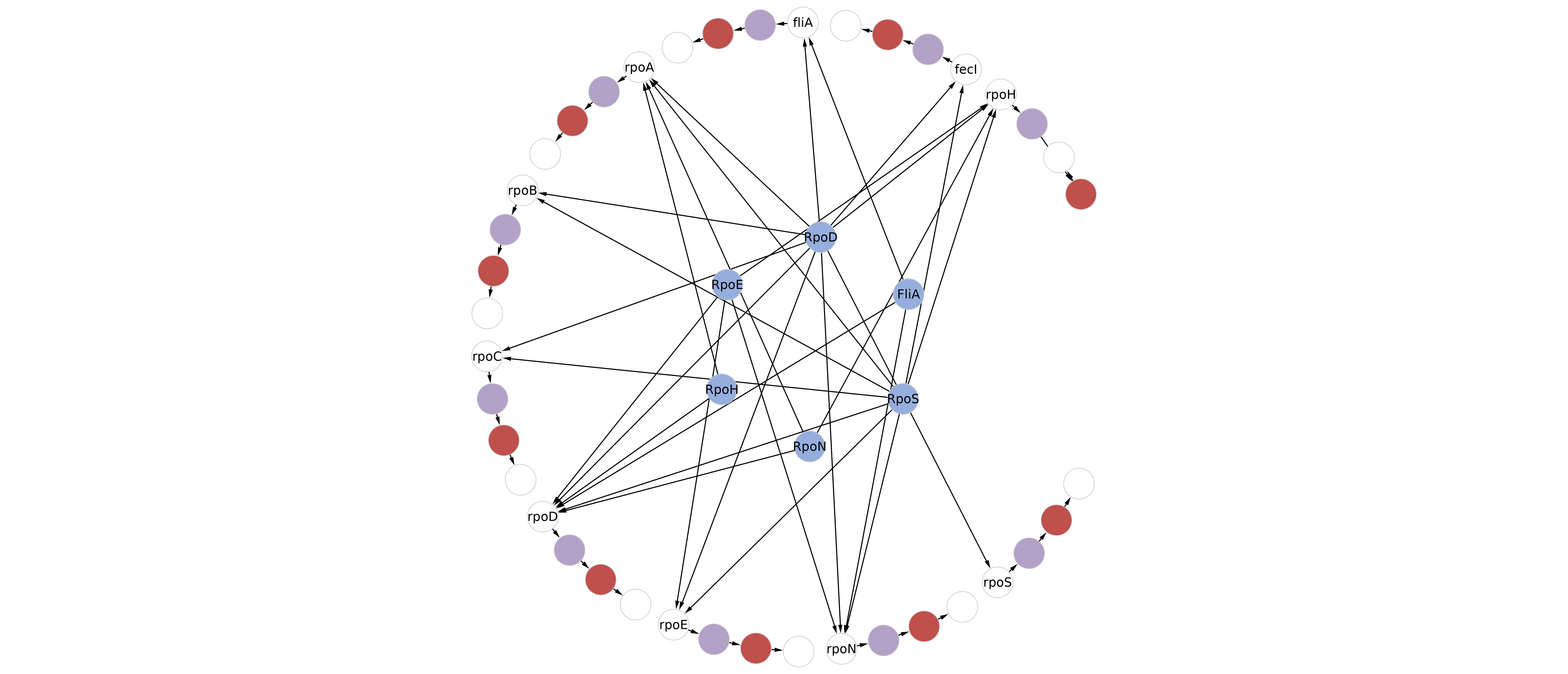
Visualization in Cytoscape. Colors and arrows remains to the user for customization. The network could be complemented with a description of sigma factor specifity for promoter, as the following network
Finally, execute the “Rules from metabolic network.ipynb” to obtain the Rules to model the defined network. If using a Sigma Factor-Promoter Interaction Network, the user could use “Rules from SigmaFactors x Architecture” to obtain the Rules to model both network at once. The complete rule-based model can be found in the arabinose folder (1st example) and in the sigma folder (2nd example) from the Network Biology Lab GitHub repository here.
Note
Kappa BioBrick Framework. Rules for transcription and translation come from the work of Stewart and Wilson-Kanamori (See more here). A “pure” genome graph use the original defined rules, while a genome graph + sigma factor specifity use a modify form to model the release of the sigma factor from the RNA Polymerase at the transcription initiation. Note the explicit modeling of the RNA Polymerase in the second example.
Rule('docking_araB_pro1',
        cplx(name = 'RNAP', dna = None) + dna(name = 'araB', type = 'pro1', prot = None, free = 'True') |
        cplx(name = 'RNAP', dna = 1) % dna(name = 'araB', type = 'pro1', prot = 1, free = 'False'),
        Parameter('fwd_docking_araB_pro1', 1), Parameter('rvs_docking_araB_pro1', 1))
OR
# [rpoA, rpoA, rpoB, rpoC, rpoD] interacts with BS_rpoA_pro1
Rule('docking_1_rpoA_pro1',
        prot(name = 'rpoA', dna = None, met = None, up = None, dw = 1) %
        prot(name = 'rpoA', dna = None, met = None, up = 1, dw = 2) %
        prot(name = 'rpoB', dna = None, met = None, up = 2, dw = 3) %
        prot(name = 'rpoC', dna = None, met = None, up = 3, dw = 4) %
        prot(name = 'rpoD', dna = None, met = None, up = 4, dw = None) +
        dna(name = 'rpoA', type = 'pro1', prot = None, free = 'True', up = WILD, dw = WILD) |
        prot(name = 'rpoA', dna = None, met = None, up = None, dw = 1) %
        prot(name = 'rpoA', dna = None, met = None, up = 1, dw = 2) %
        prot(name = 'rpoB', dna = None, met = None, up = 2, dw = 3) %
        prot(name = 'rpoC', dna = None, met = None, up = 3, dw = 4) %
        prot(name = 'rpoD', dna = 5, met = None, up = 4, dw = None) %
        dna(name = 'rpoA', type = 'pro1', prot = 5, free = 'False', up = WILD, dw = WILD),
        Parameter('fwd_docking_1_rpoA_rbs', 1),
        Parameter('rvs_docking_1_rpoA_pro1', 0))
Note
Reversibility of reactions. Atlas writes irreversible Rules for each
interaction between the RNA Polymerase and a promoter. The Parameter('rvs_ReactionName', 0))
must be set to non-zero to define a reversible reaction. The remaining Rules
are irreversible without a way to define reversible reactions.
Note
Simulation. The model can be simulated only with the instantiation of
Monomers and Initials (More here).
Run Monomer+Initials+Observables from metabolic network.ipynb to obtain
automatically the necessary Monomers and Initials (including
proteins and enzymatic complexes). For initial genes, please refer to the
following example:
Initial(
        dna(name = 'rpoB', type = 'pro1', free = 'True', prot = None, rna = None, up = None, dw = 1) %
        dna(name = 'rpoB', type = 'rbs', free = 'True', prot = None, rna = None, up = 1, dw = 2) %
        dna(name = 'rpoB', type = 'cds', free = 'True', prot = None, rna = None, up = 2, dw = 3) %
        dna(name = 'rpoC', type = 'rbs', free = 'True', prot = None, rna = None, up = 3, dw = 4) %
        dna(name = 'rpoC', type = 'cds', free = 'True', prot = None, rna = None, up = 4, dw = 5) %
        dna(name = 'rpoC', type = 'ter1', free = 'True', prot = None, rna = None, up = 5, dw = None),
        Parameter('t0_rpoBC_operon', 1))
Plotting. The model can be observed only with the instantation of
Observables (More here).
Run Monomer+Initials+Observables from metabolic network.ipynb to obtain
automatically the all possible Observables for metabolites.